Debugging

Debugging inference in RxInfer can be quite challenging, mostly due to the reactive nature of the inference, undefined order of computations, the use of observables, and generally hard-to-read stack traces in Julia. Below we discuss ways to help you find problems in your model that prevents you from getting the results you want.

Requesting a trace of messages

RxInfer provides a way that allows to save the history of the computations leading up to the computed messages and marginals in the inference procedure. This history is added on top of messages and marginals and is referred to as a Memory Addon. Below is an example explaining how you can extract this history and use it to fix a bug.

We show the application of the Memory Addon on the coin toss example from earlier in the documentation. We model the binary outcome $x$ (heads or tails) using a Bernoulli distribution, with a parameter $\theta$ that represents the probability of landing on heads. We have a Beta prior distribution for the $\theta$ parameter, with a known shape $\alpha$ and rate $\beta$ parameter.

\[\theta \sim \mathrm{Beta}(a, b)\]

\[x_i \sim \mathrm{Bernoulli}(\theta)\]

where $x_i \in {0, 1}$ are the binary observations (heads = 1, tails = 0). This is the corresponding RxInfer model:

using RxInfer, Random, Plots

n = 4
θ_real = 0.3
dataset = float.(rand(Bernoulli(θ_real), n))

@model function coin_model(x)
    θ  ~ Beta(4, huge)
    x .~ Bernoulli(θ)
end

result = infer(
    model = coin_model(),
    data  = (x = dataset, ),
)

Inference results:
  Posteriors       | available for (θ)

The model will run without errors. But when we plot the posterior distribution for $\theta$, something's wrong. The posterior seems to be a flat distribution:

rθ = range(0, 1, length = 1000)

plot(rθ, (rvar) -> pdf(result.posteriors[:θ], rvar), label="Infered posterior")
vline!([θ_real], label="Real θ", title = "Inference results")

We can figure out what's wrong by tracing the computation of the posterior with the Memory Addon. To obtain the trace, we have to add addons = (AddonMemory(),) as an argument to the inference function. Note, that the argument to the addons keyword argument must be a tuple, because multiple addons can be activated at the same time. Here, we create a tuple with a single element however.

result = infer(
    model = coin_model(),
    data  = (x = dataset, ),
    addons = (AddonMemory(),)
)

Inference results:
  Posteriors       | available for (θ)

Now we have access to the messages that led to the marginal posterior:

RxInfer.ReactiveMP.getaddons(result.posteriors[:θ])

(AddonMemory(Product memory:
 Message mapping memory:
    At the node: Beta
    Towards interface: Val{:out}()
    With local constraint: Marginalisation()
    With addons: (AddonMemory(nothing),)
    With input marginals on Val{(:a, :b)}() edges: (PointMass{Int64}(4), PointMass{TinyHugeNumbers.HugeNumber}(huge))
    With the result: Beta{Float64}(α=4.0, β=1.0e12)
 Message mapping memory:
    At the node: Bernoulli
    Towards interface: Val{:p}()
    With local constraint: Marginalisation()
    With addons: (AddonMemory(nothing),)
    With input marginals on Val{(:out,)}() edges: (PointMass{Float64}(1.0),)
    With the result: Beta{Float64}(α=2.0, β=1.0)
 Message mapping memory:
    At the node: Bernoulli
    Towards interface: Val{:p}()
    With local constraint: Marginalisation()
    With addons: (AddonMemory(nothing),)
    With input marginals on Val{(:out,)}() edges: (PointMass{Float64}(1.0),)
    With the result: Beta{Float64}(α=2.0, β=1.0)
 Message mapping memory:
    At the node: Bernoulli
    Towards interface: Val{:p}()
    With local constraint: Marginalisation()
    With addons: (AddonMemory(nothing),)
    With input marginals on Val{(:out,)}() edges: (PointMass{Float64}(1.0),)
    With the result: Beta{Float64}(α=2.0, β=1.0)
 Message mapping memory:
    At the node: Bernoulli
    Towards interface: Val{:p}()
    With local constraint: Marginalisation()
    With addons: (AddonMemory(nothing),)
    With input marginals on Val{(:out,)}() edges: (PointMass{Float64}(1.0),)
    With the result: Beta{Float64}(α=2.0, β=1.0)
),)

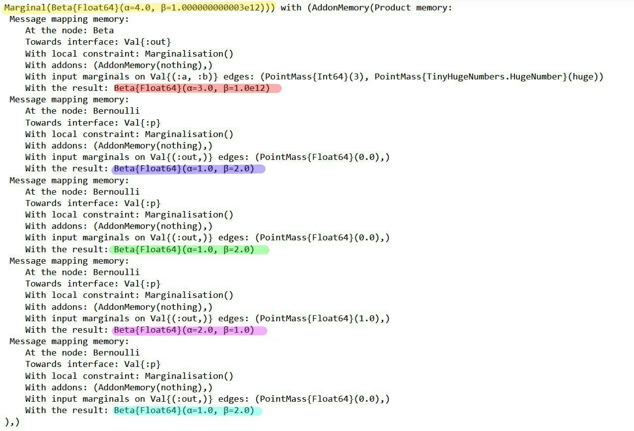
The messages in the factor graph are marked in color. If you're interested in the mathematics behind these results, consider verifying them manually using the general equation for sum-product messages:

\[\underbrace{\overrightarrow{\mu}_{θ}(θ)}_{\substack{ \text{outgoing}\\ \text{message}}} = \sum_{x_1,\ldots,x_n} \underbrace{\overrightarrow{\mu}_{X_1}(x_1)\cdots \overrightarrow{\mu}_{X_n}(x_n)}_{\substack{\text{incoming} \\ \text{messages}}} \cdot \underbrace{f(θ,x_1,\ldots,x_n)}_{\substack{\text{node}\\ \text{function}}}\]

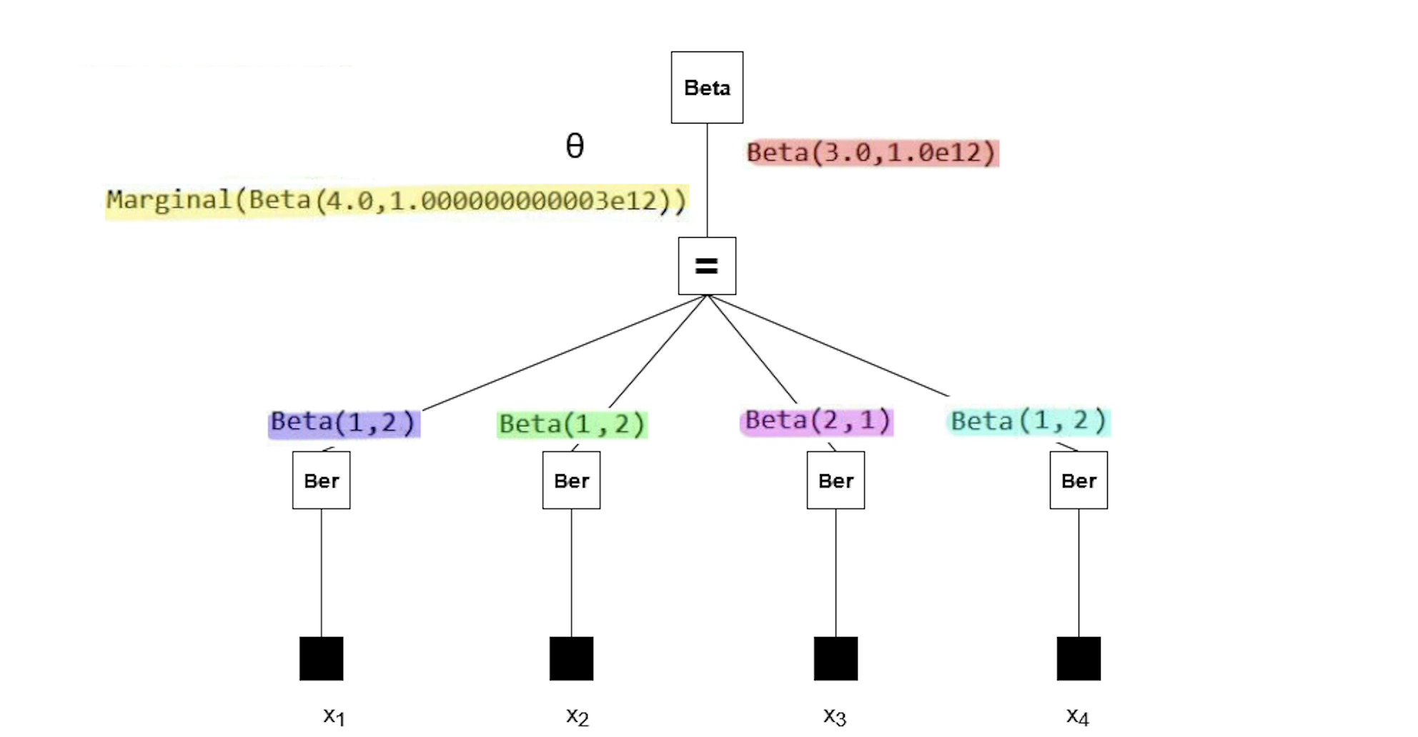
Note that the posterior (yellow) has a rate parameter on the order of 1e12. Our plot failed because a Beta distribution with such a rate parameter cannot be accurately depicted using the range of $\theta$ we used in the code block above. So why does the posterior have this rate parameter?

All the observations (purple, green, pink, blue) have much smaller rate parameters. It seems the prior distribution (red) has an unusual rate parameter, namely 1e12. If we look back at the model, the parameter was set to huge (which is a reserved keyword meaning 1e12). Reducing the prior rate parameter will ensure the posterior has a reasonable rate parameter as well.

@model function coin_model(x)
    θ  ~ Beta(4, 100)
    x .~ Bernoulli(θ)
end

result = infer(
    model = coin_model(),
    data  = (x = dataset, ),
)

Inference results:
  Posteriors       | available for (θ)

rθ = range(0, 1, length = 1000)

plot(rθ, (rvar) -> pdf(result.posteriors[:θ], rvar), fillalpha = 0.4, fill = 0, label="Infered posterior")
vline!([θ_real], label="Real θ", title = "Inference results")

Now the posterior has much more sensible shape thus confirming that we have identified the original issue correctly. We can run the model with more observations, to get an even better posterior:

result = infer(
    model = coin_model(),
    data  = (x = float.(rand(Bernoulli(θ_real), 1000)), ),
)

rθ = range(0, 1, length = 1000)
plot(rθ, (rvar) -> pdf(result.posteriors[:θ], rvar), fillalpha = 0.4, fill = 0, label="Infered posterior (1000 observations)")
vline!([θ_real], label="Real θ", title = "Inference results")

Using callbacks in the infer function

Another way to inspect the inference procedure is to use the callbacks or events from the infer function. Read more about callbacks in the documentation to the infer function. Here, we show a simple application of callbacks to a simple IID inference problem. We start with model specification:

using RxInfer

@model function iid_normal(y)
    μ  ~ Normal(mean = 0.0, variance = 100.0)
    γ  ~ Gamma(shape = 1.0, rate = 1.0)
    y .~ Normal(mean = μ, precision = γ)
end

Next, let us define a syntehtic dataset:

dataset = rand(NormalMeanPrecision(3.1415, 30.0), 100)

Now, we can use the callbacks argument of the infer function to track the order of posteriors computation and their intermediate values for each variational iteration:

# A callback that will be called every time before a variational iteration starts
function before_iteration_callback(model, iteration)
    println("Starting iteration ", iteration)
end

# A callback that will be called every time after a variational iteration finishes
function after_iteration_callback(model, iteration)
    println("Iteration ", iteration, " has been finished")
end

# A callback that will be called every time a posterior is updated
function on_marginal_update_callback(model, variable_name, posterior)
    println("Latent variable ", variable_name, " has been updated. Estimated mean is ", mean(posterior), " with standard deviation ", std(posterior))
end

on_marginal_update_callback (generic function with 1 method)

After we have defined all callbacks of interest, we can call the infer function passing them in the callback argument as a named tuple:

init = @initialization begin
    q(μ) = vague(NormalMeanVariance)
end

result = infer(
    model = iid_normal(),
    data  = (y = dataset, ),
    constraints = MeanField(),
    iterations = 5,
    initialization = init,
    returnvars = KeepLast(),
    callbacks = (
        on_marginal_update = on_marginal_update_callback,
        before_iteration   = before_iteration_callback,
        after_iteration    = after_iteration_callback
    )
)

Starting iteration 1
Latent variable γ has been updated. Estimated mean is 1.0199999999900495e-12 with standard deviation 1.4282856856946363e-13
Latent variable μ has been updated. Estimated mean is 3.178081906763656e-8 with standard deviation 9.999999948999998
Iteration 1 has been finished
Starting iteration 2
Latent variable γ has been updated. Estimated mean is 0.009293366510008054 with standard deviation 0.001301331603753717
Latent variable μ has been updated. Estimated mean is 3.0825967461497723 with standard deviation 1.0317853710383051
Iteration 2 has been finished
Starting iteration 3
Latent variable γ has been updated. Estimated mean is 0.9161237517451043 with standard deviation 0.12828298440736902
Latent variable μ has been updated. Estimated mean is 3.115426540944902 with standard deviation 0.10447183596932388
Iteration 3 has been finished
Starting iteration 4
Latent variable γ has been updated. Estimated mean is 17.400238019218673 with standard deviation 2.4365206755658897
Latent variable μ has been updated. Estimated mean is 3.115748700712917 with standard deviation 0.02397293222161216
Iteration 4 has been finished
Starting iteration 5
Latent variable γ has been updated. Estimated mean is 21.12671268156042 with standard deviation 2.9583315008971045
Latent variable μ has been updated. Estimated mean is 3.115751859144151 with standard deviation 0.021756198327312227
Iteration 5 has been finished

We can see that the callback has been correctly executed for each intermediate variational iteration.

println("Estimated mean: ", mean(result.posteriors[:μ]))
println("Estimated precision: ", mean(result.posteriors[:γ]))

Estimated mean: 3.115751859144151
Estimated precision: 21.12671268156042

Using LoggerPipelineStage

ReactiveMP inference engine allows attaching extra computations to the default computational pipeline of message passing. Read more about pipelines in the corresponding section of ReactiveMP. Here we show how to use LoggerPipelineStage to trace the order of message passing updates for debugging purposes. We start with model specification:

using RxInfer

@model function iid_normal_with_pipeline(y)
    μ  ~ Normal(mean = 0.0, variance = 100.0)
    γ  ~ Gamma(shape = 1.0, rate = 1.0)
    y .~ Normal(mean = μ, precision = γ) where { pipeline = LoggerPipelineStage() }
end

Next, let us define a syntehtic dataset:

# We use less data points in the dataset to reduce the amount of text printed
# during the inference
dataset = rand(NormalMeanPrecision(3.1415, 30.0), 5)

Now, we can call the infer function. We combine the pipeline logger stage with the callbacks, which were introduced in the previous section:

result = infer(
    model = iid_normal_with_pipeline(),
    data  = (y = dataset, ),
    constraints = MeanField(),
    iterations = 5,
    initialization = init,
    returnvars = KeepLast(),
    callbacks = (
        on_marginal_update = on_marginal_update_callback,
        before_iteration   = before_iteration_callback,
        after_iteration    = after_iteration_callback
    )
)

Starting iteration 1
[Log][NormalMeanPrecision][τ]: DeferredMessage([ use `as_message` to compute the message ])
[Log][NormalMeanPrecision][τ]: DeferredMessage([ use `as_message` to compute the message ])
[Log][NormalMeanPrecision][τ]: DeferredMessage([ use `as_message` to compute the message ])
[Log][NormalMeanPrecision][τ]: DeferredMessage([ use `as_message` to compute the message ])
[Log][NormalMeanPrecision][τ]: DeferredMessage([ use `as_message` to compute the message ])
Latent variable γ has been updated. Estimated mean is 1.399999999986072e-12 with standard deviation 7.483314773473434e-13
[Log][NormalMeanPrecision][μ]: DeferredMessage([ use `as_message` to compute the message ])
[Log][NormalMeanPrecision][μ]: DeferredMessage([ use `as_message` to compute the message ])
[Log][NormalMeanPrecision][μ]: DeferredMessage([ use `as_message` to compute the message ])
[Log][NormalMeanPrecision][μ]: DeferredMessage([ use `as_message` to compute the message ])
[Log][NormalMeanPrecision][μ]: DeferredMessage([ use `as_message` to compute the message ])
Latent variable μ has been updated. Estimated mean is 2.159580897294956e-9 with standard deviation 9.9999999965
Iteration 1 has been finished
Starting iteration 2
[Log][NormalMeanPrecision][τ]: DeferredMessage([ use `as_message` to compute the message ])
[Log][NormalMeanPrecision][τ]: DeferredMessage([ use `as_message` to compute the message ])
[Log][NormalMeanPrecision][τ]: DeferredMessage([ use `as_message` to compute the message ])
[Log][NormalMeanPrecision][τ]: DeferredMessage([ use `as_message` to compute the message ])
[Log][NormalMeanPrecision][τ]: DeferredMessage([ use `as_message` to compute the message ])
Latent variable γ has been updated. Estimated mean is 0.012733213655948516 with standard deviation 0.006806188990450083
[Log][NormalMeanPrecision][μ]: DeferredMessage([ use `as_message` to compute the message ])
[Log][NormalMeanPrecision][μ]: DeferredMessage([ use `as_message` to compute the message ])
[Log][NormalMeanPrecision][μ]: DeferredMessage([ use `as_message` to compute the message ])
[Log][NormalMeanPrecision][μ]: DeferredMessage([ use `as_message` to compute the message ])
[Log][NormalMeanPrecision][μ]: DeferredMessage([ use `as_message` to compute the message ])
Latent variable μ has been updated. Estimated mean is 2.6663181991606226 with standard deviation 3.6843955949358724
Iteration 2 has been finished
Starting iteration 3
[Log][NormalMeanPrecision][τ]: DeferredMessage([ use `as_message` to compute the message ])
[Log][NormalMeanPrecision][τ]: DeferredMessage([ use `as_message` to compute the message ])
[Log][NormalMeanPrecision][τ]: DeferredMessage([ use `as_message` to compute the message ])
[Log][NormalMeanPrecision][τ]: DeferredMessage([ use `as_message` to compute the message ])
[Log][NormalMeanPrecision][τ]: DeferredMessage([ use `as_message` to compute the message ])
Latent variable γ has been updated. Estimated mean is 0.09872433003583993 with standard deviation 0.052770374104701284
[Log][NormalMeanPrecision][μ]: DeferredMessage([ use `as_message` to compute the message ])
[Log][NormalMeanPrecision][μ]: DeferredMessage([ use `as_message` to compute the message ])
[Log][NormalMeanPrecision][μ]: DeferredMessage([ use `as_message` to compute the message ])
[Log][NormalMeanPrecision][μ]: DeferredMessage([ use `as_message` to compute the message ])
[Log][NormalMeanPrecision][μ]: DeferredMessage([ use `as_message` to compute the message ])
Latent variable μ has been updated. Estimated mean is 3.0238569727768505 with standard deviation 1.4091194326613024
Iteration 3 has been finished
Starting iteration 4
[Log][NormalMeanPrecision][τ]: DeferredMessage([ use `as_message` to compute the message ])
[Log][NormalMeanPrecision][τ]: DeferredMessage([ use `as_message` to compute the message ])
[Log][NormalMeanPrecision][τ]: DeferredMessage([ use `as_message` to compute the message ])
[Log][NormalMeanPrecision][τ]: DeferredMessage([ use `as_message` to compute the message ])
[Log][NormalMeanPrecision][τ]: DeferredMessage([ use `as_message` to compute the message ])
Latent variable γ has been updated. Estimated mean is 0.5784862083116619 with standard deviation 0.3092138849251684
[Log][NormalMeanPrecision][μ]: DeferredMessage([ use `as_message` to compute the message ])
[Log][NormalMeanPrecision][μ]: DeferredMessage([ use `as_message` to compute the message ])
[Log][NormalMeanPrecision][μ]: DeferredMessage([ use `as_message` to compute the message ])
[Log][NormalMeanPrecision][μ]: DeferredMessage([ use `as_message` to compute the message ])
[Log][NormalMeanPrecision][μ]: DeferredMessage([ use `as_message` to compute the message ])
Latent variable μ has been updated. Estimated mean is 3.074486150741329 with standard deviation 0.5869742436778188
Iteration 4 has been finished
Starting iteration 5
[Log][NormalMeanPrecision][τ]: DeferredMessage([ use `as_message` to compute the message ])
[Log][NormalMeanPrecision][τ]: DeferredMessage([ use `as_message` to compute the message ])
[Log][NormalMeanPrecision][τ]: DeferredMessage([ use `as_message` to compute the message ])
[Log][NormalMeanPrecision][τ]: DeferredMessage([ use `as_message` to compute the message ])
[Log][NormalMeanPrecision][τ]: DeferredMessage([ use `as_message` to compute the message ])
Latent variable γ has been updated. Estimated mean is 1.8055404305303777 with standard deviation 0.9651019555732843
[Log][NormalMeanPrecision][μ]: DeferredMessage([ use `as_message` to compute the message ])
[Log][NormalMeanPrecision][μ]: DeferredMessage([ use `as_message` to compute the message ])
[Log][NormalMeanPrecision][μ]: DeferredMessage([ use `as_message` to compute the message ])
[Log][NormalMeanPrecision][μ]: DeferredMessage([ use `as_message` to compute the message ])
[Log][NormalMeanPrecision][μ]: DeferredMessage([ use `as_message` to compute the message ])
Latent variable μ has been updated. Estimated mean is 3.0817019635992535 with standard deviation 0.33263733129075257
Iteration 5 has been finished

We can see the order of message update events. Note that ReactiveMP may decide to compute messages lazily, in which case the actual computation of the value of a message will be deffered until later moment. In this case, LoggerPipelineStage will report DefferedMessage.